Hey everyone,
HAPPY TUESDAY!!!!!!
I wanted to share some useful ways to add cells in excel
that can increase efficiency in any kind of analysis or summing type situation.
I’m providing this example for demonstration purposes, but
you can apply these techniques to a number of different scenarios in excel. The
SUMIF and SUMIFS formulas can be used with more types of data than a Pivot
Table, however if the data’s in the right format, Pivot Tables are much more
versatile and powerful than the SUMIF and SUMIFS formulas.
Example: take a list of numbers that we want to summarize in
a certain way. Here I have a list of names, dates, numbers, and type of animal.
Let’s say this is a list of how many cats or dogs each person adopted on each
day.

Now, if we want to add up the total number of cats and total
number of dogs that Sally adopted during this time period, there are a few ways
we can do this:
Five Different ways to add:
1.
Ten-key / adding in the cell
2.
Using an Equals and Plus cell reference formula
3.
Adding a flag and using a Sumif formula
4.
Using a Sumifs formula
5.
Using a pivot table
Breakdown:
Ten-key:
a. How: use the ten-key on your desk, a
calculator app on your computer, or add within the cell (6+5+1+8 = 20)
b. Analysis: While this is a reliable and
tried & true method, it’s arguably the least efficient, especially when you
start getting past 50 items or so (depending on how speedy you are with the
ten-key)
Equals and Plus formula.
a. How: use a formula in another cell. In
the above example, the formula for Sally’s Cats would be “=C11+C17+C19+C29”
b. Analysis: While this seems easy, it’s
still a lot of manual work, and almost as inefficient as using the ten-key.
Also if you miss one, it’s not very easy to tell which cells you might have
missed, again especially if you have over 50 rows of data. Also this one is a
little too “clicky typey” for me.
Flag and a Sumif formula:
a. How: Add a “flag” such as a number or
character in the row to the right of the numbers you want to add. For example,
see below:

§ The
SUMIF formula has three parts*: (range, criteria,
[sum range])
§ The
“range” tells the formula which cells to look for the matching criteria.
§ The
“criteria” tells the formula what to look for within the range.
§ The
“sum range” is the range we want to add if the “range” cell in the same row
meets the “criteria”
§ Next
add this formula in the resulting cell to calculate the Sally Cat sum: =SUMIF(E:E,”1”,C:C)

* Excel expert note:
The “sum range” is optional. If left out, the “range” becomes the “sum range”.
But I usually specify the “sum range”, as my “range” usually is not the same
column as my “sum range”. Leaving the “range” as the “sum range” is useful if
you do a sumif that includes a formula criteria on numbers that you also want
to sum. For example you could SumIf a list of numbers on only those numbers
that are greater than 5.
b. Analysis: SUMIF can be much more
efficient than the previous two methods. But it can be even more helpful in
that if you add the formula before adding the flags, you can watch the formula
balance increase or decrease as you add or remove flags from the different rows.
Try it out! The downside is there’s
still a manual element to this, which involves going in and adding the ‘1’s and
‘2’s next to every row you want to include.
c. Additional note: The second part of the
formula, the “criteria”, can reference a cell that contains the specified
criteria instead of hardcoding the criteria. For example, see below to easily
add up the Sally Cat and Sally Dog amounts using this formula in I3: =SUMIF(E:E,H2,C:C) and
this formula in I4: =SUMIF(E:E,H3,C:C)

Here’s with the formulas showing:

As
you can see, SUMIF with reference to a cell for criteria is very useful because
you can add additional flags all day long, and just copy and paste your SUMIF
formula.
SUMIFS formula:
a.
How: The
SUMIFS formula will only work if you have reliable and consistent data, in the
exact same format throughout the data. If you do, this is a fantastic way to
add numbers using multiple criteria. The two criteria we are using here are
Name (Sally) and Type (either Dog or Cat).
·
This one gets a little more complex, but I promise
it is easier once you understand how it works.
· The
SUMIFS formula, like the SUMIF formula, involves RANGE, CRITERIA, and SUM
RANGE. However with the SUMIFS, you can have MORE THAN ONE criteria. It’s
organized as follows: (sum range, criteria
range1, criteria1, [criteria range 2, criteria 2], etc……)
·
Given our Sally Cat calculation, we’d use the
following formula: =SUMIFS(C:C, D:D,"Cat",A:A, "Sally")
·
And yes, you guessed it, to add up the Sally
Dogs just replace the word “Cat” with the word “Dog”

Here’s with the formulas

·
And again, you can use formulas to reference the
cells containing “Cat”, “Dog”, and “Sally”:

·
(Note the Dollar
sign ‘$’ in the formula: This is used to keep the ‘H’ and the ‘2’ the same even
when the formula is copied and pasted to different rows or columns)
·
(Fun tip: CTRL+~ is
a shortcut to show all formulas in excel. Press it again to hide formulas.)
b.
Analysis:
If data is in a consistent format, this is great way to do multi-conditional
sumifs. I used to use these quite a lot, however I graduated to pivot tables a
few years ago...
Pivot Tables
a.
How: There
are several things you must do before creating a pivot table:
·
First, make sure your data is correctly
formatted. No blank columns, no blank rows, and all columns must have a label,
preferably unique. The example above is almost ready to go, except it has no
header for the Names, therefore we must add a header (I used “Name” in cell A1)
·
Next select the data you want to include in the
pivot table. In our example, it’s A1:D29.
You can select it by pressing CTRL+A anywhere within the data, just look
to make sure it correctly highlighted what you want. Here’s what it should look
like:

·
Now go to INSERT > Pivot Table
·
Make sure the correct Table/Range is selected,
and the New Worksheet is selected, then hit OK.

·
Now we have a Pivot Table, but note nothing
shows up until we tell excel what data goes where:

·
Definitions:
1. Here’s
where the pivot table results will go
2. These
are the columns, or Fields, that we pulled into the pivot table data. To create
the pivot table, we must pull several of these Fields into one of the four areas
in the bottom right quadrant. Typically you at least will want to have ROWS and
VALUES.
3. Filters
are used to filter the results.
4. Columns
take the data in whatever PivotTable Filed you want to display as columns.
Easier to understand this one when you
see it in action
5. Rows
are my favorite. These are used to setup what we will summarize results on
later, and we will use the RANGE from the SUMIF formula for the rows
6. Values
take the Field input, and summarize or count based on the ROWS and COLUMNS that
match. Again this makes more sense when you see it, but I’ll show how we can
create a pivot table that gives us exactly what we created using the sumifs
formula.
·
Setting up the pivot table to mimic the SUMIFS
(to move, click and drag the fields from the top area to the bottom quadrant):
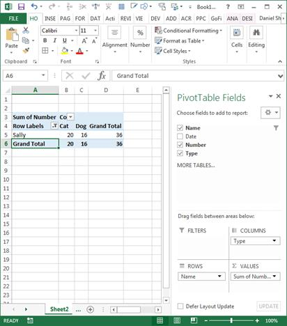
1. Put
Name in ROWS
2. Type
goes in COLUMNS
3. Number
goes in VALUES (make sure it is “SUM” rather than “COUNT”)
4. Date
is not important to us at this point so we will not use it.

·
Note how easily we can now see the total cats
and dogs for each person!
·
Now if we want to just see Sally’s you can
filter using the dropdown arrow next to “Row Labels”, uncheck “select all”, and
check Sally.

Click “OK” and
BOOM!
b.
Analysis:
In my opinion, pivot tables are clearly the best here, as they provide a
very versatile and easy to use format. The data can be literally “pivoted” in
different directions, filtered in different ways, with ease.
Cheers!
Daniel
No comments:
Post a Comment